Case study: Citizen science phosphate data comparisons
The purpose of this case study is to use the Oxford Rivers Portal API to compare phosphate water-quality measurements made by the Environment Agency (EA) and the River Thames Initiative (TI) with citizen science measurements made by FreshWater Watch (FWW).
Method
Every FWW measurement will be paired with its nearest (both spatially and temporally) EA water quality (EA WQ) measurements and TI measurements. A spatial limit of 100 m and a temporal limit of 24 hours will be applied when matching nearest measurements. After matching, the EA WQ and TI data will be compared to assess reliability of this matching method. Finally, the FWW data will be compared in turn to both the TI and EA datasets.
Code
1. Download libraries
Code
#librariesimport requestsimport pandas as pdpd.options.mode.chained_assignment =Noneimport seaborn as snsimport numpy as npimport geopandas as gpdfrom matplotlib import pyplot as pltfrom matplotlib.dates import DateFormatterfrom scipy.stats import pearsonr
2. Download FWW sampling sites using the API
Code
# The data is returned as JSONresponse = requests.get("https://oxfordrivers.ceh.ac.uk/getSites?datasetID=freshwater_watch")# we need to flatten the JSON to read it into pandas, this is done with JSON normalise# we set the record path to features to extract the datafww_sites = pd.json_normalize(response.json(), record_path='features')# convert to a geopandas dataframe for spatial processingfww_sites = gpd.GeoDataFrame(fww_sites)# create a geometry columnfww_sites['geometry.coordinates'] = gpd.points_from_xy(pd.DataFrame(fww_sites["geometry.coordinates"].to_list())[0], pd.DataFrame(fww_sites["geometry.coordinates"].to_list())[1])fww_sites.set_geometry('geometry.coordinates', inplace=True)fww_sites
type
geometry.type
geometry.coordinates
properties.id
properties.name
0
Feature
Point
POINT (-0.99193 51.41265)
Kybes Lane, Faudry Brook
Kybes Lane, Faudry Brook
1
Feature
Point
POINT (-0.99174 51.41106)
Kybes Lane, Foudry Brook
Kybes Lane, Foudry Brook
2
Feature
Point
POINT (-0.99193 51.41265)
Kybes Lane, Foudry Brook
Kybes Lane, Foudry Brook
3
Feature
Point
POINT (-0.99193 51.41265)
Kybes Lane, Foudry Brook
Kybes Lane, Foudry Brook
4
Feature
Point
POINT (-0.99193 51.41265)
Kybes Lane, Foudry Brook
Kybes Lane, Foudry Brook
...
...
...
...
...
...
995
Feature
Point
POINT (-1.36302 51.87284)
Wootton 3 Dorn Glyme confluence
Wootton 3 Dorn Glyme confluence
996
Feature
Point
POINT (-1.59573 51.88343)
PF5
PF5
997
Feature
Point
POINT (-1.59615 51.87934)
PF4
PF4
998
Feature
Point
POINT (-1.61841 51.89128)
PF3
PF3
999
Feature
Point
POINT (-1.61836 51.88799)
PF1
PF1
1000 rows × 5 columns
3. Download EA WQ sampling sites using the API
Code
# the data is returned as JSONresponse = requests.get("https://oxfordrivers.ceh.ac.uk/getSites?datasetID=ea_water_quality")# we need to flatten the JSON to read it into pandas, this is done with JSON normalise # we set the record path to features to extract the dataeawq_sites = pd.json_normalize(response.json(), record_path='features')# convert to a geopandas dataframe for spatial procesisngeawq_sites = gpd.GeoDataFrame(eawq_sites)# create a geometry columneawq_sites['geometry.coordinates'] = gpd.points_from_xy(pd.DataFrame(eawq_sites["geometry.coordinates"].to_list())[0], pd.DataFrame(eawq_sites["geometry.coordinates"].to_list())[1])eawq_sites.set_geometry('geometry.coordinates', inplace=True)eawq_sites
type
geometry.type
geometry.coordinates
properties.id
properties.name
properties.determinand_labels
properties.determinand_ids
0
Feature
Point
POINT (-0.53237 51.40169)
TH-PRTS0035
CHERTSEY BOURNE, U/S INTERSECTION
[Mercury - Hg, Cadmium - Cd, N Oxidised, Nitra...
[0105, 0108, 0116, 0117, 0118, 0162, 0172, 018...
1
Feature
Point
POINT (-0.52085 51.41779)
TH-PRTS0038
MEAD LAKE DITCH, U/S INTERSECTION
[Mercury - Hg, Cadmium - Cd, N Oxidised, Nitra...
[0105, 0108, 0116, 0117, 0118, 0162, 0172, 018...
2
Feature
Point
POINT (-0.51563 51.41127)
TH-PRTS0044
MEAD LAKE DITCH, D/S INTERSECTION
[Mercury - Hg, Cadmium - Cd, N Oxidised, Nitra...
[0105, 0108, 0116, 0117, 0118, 0162, 0172, 018...
3
Feature
Point
POINT (-0.51227 51.41949)
TH-PRTS0045
THAMES D/S OF RUNNYMEDE CHANNEL INTAKE
[Mercury - Hg, Cadmium - Cd, N Oxidised, Nitra...
[0105, 0108, 0116, 0117, 0118, 0162, 0172, 018...
4
Feature
Point
POINT (-0.51009 51.42274)
TH-PRTS0046
THAMES U/S OF RUNNYMEDE CHANNEL INTAKE
[Mercury - Hg, Cadmium - Cd, Nitrate-N, Sulpha...
[0105, 0108, 0117, 0183, 0192, 0207, 0237, 024...
...
...
...
...
...
...
...
...
475
Feature
Point
POINT (-0.1953 51.09866)
TH-PMLR0251
BROADFIELD BROOK ABOVE OUTFALL, BROADFIE
[O Diss %sat, Oxygen Diss]
[9901, 9924]
476
Feature
Point
POINT (-0.22412 51.09586)
TH-PMLR0289
DOUSTER BROOK, BELOW DOUSTER POND
[O Diss %sat, Oxygen Diss]
[9901, 9924]
477
Feature
Point
POINT (-0.24428 51.09149)
TH-PMLR0290
IFIELD BROOK BELOW FOXHOLE POND
[O Diss %sat, Oxygen Diss]
[9901, 9924]
478
Feature
Point
POINT (-0.54948 51.45739)
TH-PRTS0019
WRAYSBURY II (S)
[O Diss %sat, Oxygen Diss]
[9901, 9924]
479
Feature
Point
POINT (-0.53963 51.46806)
TH-PRTS0030
MILDRIDGE GREEN DRAIN
[Oxygen Diss]
[9924]
480 rows × 7 columns
4. Download the TI sampling sites using an API
Code
# the data is returned as JSONresponse = requests.get("https://oxfordrivers.ceh.ac.uk/getSites?datasetID=thames_initiative")# we need to flatten the JSON to read it into pandas, this is done with JSON normalise# we set the record path to features to extract the data. thamesinit_sites = pd.json_normalize(response.json(), record_path='features')# convert to a geopandas dataframe for spatial procesisngthamesinit_sites = gpd.GeoDataFrame(thamesinit_sites)# create a geometry columnthamesinit_sites['geometry.coordinates'] = gpd.points_from_xy(pd.DataFrame(thamesinit_sites["geometry.coordinates"].to_list())[0], pd.DataFrame(thamesinit_sites["geometry.coordinates"].to_list())[1])thamesinit_sites.set_geometry('geometry.coordinates', inplace=True)thamesinit_sites
type
geometry.type
geometry.coordinates
properties.id
properties.name
properties.code
0
Feature
Point
POINT (-1.11507 51.74037)
Thame at Wheatley
Thame at Wheatley
TC1
1
Feature
Point
POINT (-1.23681 51.82125)
Ray at Islip
Ray at Islip
TC2
2
Feature
Point
POINT (-1.27724 51.83319)
Cherwell at Hampton Poyle
Cherwell at Hampton Poyle
TC3
3
Feature
Point
POINT (-1.69767 51.68038)
Cole at Lyte Bridge
Cole at Lyte Bridge
TC9
4
Feature
Point
POINT (-1.28567 51.6669)
Ock at Abingdon
Ock at Abingdon
TC11
5
Feature
Point
POINT (-1.0858 51.4677)
Pang at Tidmarsh
Pang at Tidmarsh
TC12
6
Feature
Point
POINT (-0.75007 51.47809)
The Cut at Paley Street
The Cut at Paley Street
TC15
7
Feature
Point
POINT (-0.55397 51.44077)
Thames at Runnymede
Thames at Runnymede
TC16
8
Feature
Point
POINT (-1.12199 51.60735)
Thames at Wallingford
Thames at Wallingford
TC18
9
Feature
Point
POINT (-1.17921 51.39646)
Kennet at Woolhampton
Kennet at Woolhampton
TC20
10
Feature
Point
POINT (-1.18381 51.38031)
Enborne at Brimpton
Enborne at Brimpton
TC21
11
Feature
Point
POINT (-0.6973 51.53936)
Thames at Taplow
Thames at Taplow
TC27
5. Convert geometries
Convert the geometries from WGS 84 degree based projection to the British National Grid 27700 projection. The units of the latter projection are meters, which makes it easier to define a spatial radius to match samples within.
Get timeseries data for each site and match spatially joined measurements that are within 24 hours of each other.
Code
# match samples that occur within 24 hours of one anothermerged_timeseries_eawq_ti = pd.DataFrame()# process one site at a timefor idx in merged_sites_wq_ti.index:# download the thames initiative time series data response = requests.get(f"https://oxfordrivers.ceh.ac.uk/getTimeseries?siteID={merged_sites_wq_ti.loc[idx,'properties.id_right']}&datasetID=thames_initiative&determinand=Soluble%20reactive%20phosphorus%20(%CE%BCg/L)") ti_timeseries=pd.json_normalize(response.json(), record_path ='data')#format the timeseries as a dataframeiflen(ti_timeseries) >0: ti_timeseries['dti'] = pd.DatetimeIndex(ti_timeseries['datetime']) ti_timeseries.loc[ti_timeseries['value'] =='','value'] = np.nan #set missing values to nan ti_timeseries.loc[ti_timeseries['value'] =='No Sample','value'] = np.nan #set missing values to nan ti_timeseries['value'] = ti_timeseries['value'].astype('float') ti_timeseries['value'] = ti_timeseries['value']/1000#ug to mg ti_timeseries['date'] = ti_timeseries['dti'].dt.date ti_timeseries['jul2'] = pd.DatetimeIndex(ti_timeseries['dti']).to_julian_date() ti_timeseries['site'] = merged_sites_wq_ti.loc[idx,'properties.id_right'] ti_timeseries['distance'] = merged_sites_wq_ti.loc[idx,'distance']# download the ea wq time series data response = requests.get(f"https://oxfordrivers.ceh.ac.uk/getTimeseries?siteID={merged_sites_wq_ti.loc[idx,'properties.id_left']}&datasetID=ea_water_quality&determinand=0180") eawq_timeseries=pd.json_normalize(response.json(), record_path ='data')# format the timeseries as a dataframeiflen(eawq_timeseries)>0: eawq_timeseries['dti'] = pd.DatetimeIndex(eawq_timeseries['datetime']) eawq_timeseries['date'] = eawq_timeseries['dti'].dt.date eawq_timeseries['jul2'] = pd.DatetimeIndex(eawq_timeseries['dti']).to_julian_date() eawq_timeseries['site'] = merged_sites_wq_ti.loc[idx,'properties.id_left']# merge the ea wq and ti timeseries based on sampling time# tolerance 1 = 1 day = 24 hours merged_timeseries_eawq_ti = pd.concat([merged_timeseries_eawq_ti,pd.merge_asof(ti_timeseries.sort_values('jul2'),eawq_timeseries.sort_values('jul2'), left_on='jul2', right_on='jul2', direction='nearest', tolerance=1)])# calculate how far apart the samples were in timemerged_timeseries_eawq_ti['timedelta'] = merged_timeseries_eawq_ti['dti_x'] - merged_timeseries_eawq_ti['dti_y']merged_timeseries_eawq_ti=merged_timeseries_eawq_ti.filter(['value_x','value_y','dti_x','dti_y','site_x','site_y', 'distance', 'timedelta'])merged_timeseries_eawq_ti=merged_timeseries_eawq_ti.rename(columns={'value_x':'ti_value', 'value_y':'eawq_value','dti_x':'ti_dti','dti_y':'eawq_dti','site_x':'ti_site','site_y':'eawq_site'})merged_timeseries_eawq_ti = merged_timeseries_eawq_ti[merged_timeseries_eawq_ti['eawq_value'].notnull()]merged_timeseries_eawq_ti['hours_diff'] =abs(merged_timeseries_eawq_ti['timedelta'].dt.total_seconds()/3600)
Figures
Code
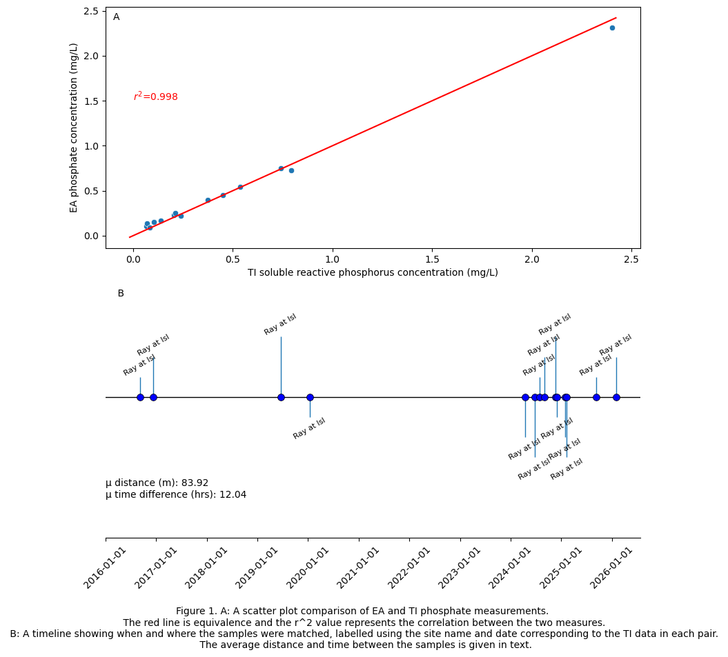
fig, axes=plt.subplots(nrows=2)fig.set_size_inches(10,10)#scatter plotsns.scatterplot(x='ti_value',y='eawq_value',data=merged_timeseries_eawq_ti, ax=axes[0])axes[0].set_ylabel('EA phosphate concentration (mg/L)')axes[0].set_xlabel('TI soluble reactive phosphorus concentration (mg/L)')#ax.set_ylim(0,0.4)x0, x1 = axes[0].get_xlim()y0, y1 = axes[0].get_ylim()lims = [max(x0, y0), min(x1, y1)]axes[0].plot(lims, lims, '-r')r, p = pearsonr(merged_timeseries_eawq_ti['ti_value'], merged_timeseries_eawq_ti['eawq_value'])r2 = r**2axes[0].text(x=0,y=1.5,s=r"$r^{2}$"+f"={np.round(r2,3)}",c='red')axes[0].text(x=-.1,y=2.4,s="A")# make a timeline# Sort by ti_dtidf =merged_timeseries_eawq_ti.sort_values(by='ti_dti')# stagger the stems levels = [1, 2, 3, -1, -2, -3] *len(df)levels = levels[:len(df)]# Draw horizontal lineaxes[1].axhline(0, color='black', linewidth=1)# Draw stems and pointssns.scatterplot(ax=axes[1],x='ti_dti', y=[0]*len(df), color='blue', s=50, zorder=3,data=df, legend=False, edgecolor='k')ci =0for i in df.index:if pd.notna(df.loc[i,'ti_dti']): axes[1].vlines(df.loc[i,'ti_dti'], 0, levels[ci], linewidth=1) ci +=1# Ensure annotations aren't too longdf['annot'] = df["ti_site"].str.slice(0,10)# Annotate each pointfor d, l, sname, di, hd inzip(df['ti_dti'], levels, df['annot'],df['distance'],df['hours_diff']): di = np.round(di,2) hd = np.round(hd,2) axes[1].text(d, l, f"{sname}", ha='center', va='bottom'if l >0else'top', fontsize=8, rotation=30)# Format x-axisaxes[1].xaxis.set_major_formatter(DateFormatter('%Y-%m-%d'))# Remove y-axis axes[1].get_yaxis().set_visible(False)#remove some spinesaxes[1].spines[["left", "top", "right"]].set_visible(False)axes[1].set_ylim([-7,5])axes[1].set_xticks(ticks=axes[1].get_xticks(),rotation=45,labels=axes[1].get_xticklabels())axes[1].set_xlabel("")axes[1].text(x=axes[1].get_xticks()[0],y=-5,s=f"μ distance (m): { np.round(df['distance'].mean(),2)}\nμ time difference (hrs): { np.round(df['hours_diff'].mean(),2)}")axes[1].text(x=axes[1].get_xticks()[0],y=5,s=f" B")fig.text(.5, -.05, "Figure 1. A: A scatter plot comparison of EA and TI phosphate measurements. \n The red line is equivalence and the r^2 value represents the correlation between the two measures. \n B: A timeline showing when and where the samples were matched, labelled using the site name and date corresponding to the TI data in each pair. \n The average distance and time between the samples is given in text.", ha='center')
Text(0.5, -0.05, 'Figure 1. A: A scatter plot comparison of EA and TI phosphate measurements. \n The red line is equivalence and the r^2 value represents the correlation between the two measures. \n B: A timeline showing when and where the samples were matched, labelled using the site name and date corresponding to the TI data in each pair. \n The average distance and time between the samples is given in text.')
Interpretation
We matched 14 samples from one site (Ray at Islip) between EA and TI datasets, the average spatial distance between the samples was 83 m and average time difference was 12 hours. There were matched samples from 2016 to 2026, with most samples matching in the period 2024–2026.
Comparing the matched values we see strong agreement, with an R^2 value of 0.998. This suggests our criteria for matching samples (within 100 m and 24 hours) is valid. However, one caveat is that samples only matched at one location, so we cannot be sure that this agreement would hold at all sites.
Comparison of TI and FWW Phosphate data
Matching samples
Code
merged_timeseries_fww_ti = pd.DataFrame()for idx in merged_sites_fww_ti.index:# download the thames initiative (ti) timeseries data response = requests.get(f"https://oxfordrivers.ceh.ac.uk/getTimeseries?siteID={merged_sites_fww_ti.loc[idx,'properties.id_right']}&datasetID=thames_initiative&determinand=Soluble%20reactive%20phosphorus%20(%CE%BCg/L)") ti_timeseries=pd.json_normalize(response.json(), record_path ='data')# format the ti data as a pandas dataframeiflen(ti_timeseries) >0: ti_timeseries['dti'] = pd.DatetimeIndex(ti_timeseries['datetime']) ti_timeseries.loc[ti_timeseries['value'] =='','value'] = np.nan #set missing values to nan ti_timeseries.loc[ti_timeseries['value'] =='No Sample','value'] = np.nan #set missing values to nan ti_timeseries['value'] = ti_timeseries['value'].astype('float') ti_timeseries['value'] = ti_timeseries['value']/1000#ug to mg ti_timeseries['date'] = ti_timeseries['dti'].dt.date ti_timeseries['jul2'] = pd.DatetimeIndex(ti_timeseries['dti']).to_julian_date() ti_timeseries['site'] = merged_sites_fww_ti.loc[idx,'properties.id_right'] ti_timeseries['distance'] = merged_sites_fww_ti.loc[idx,'distance']# download the FreshWater Watch (fww) timeseries data response = requests.get(f"https://oxfordrivers.ceh.ac.uk/getTimeseries?siteID={merged_sites_fww_ti.loc[idx,'properties.id_left']}&datasetID=freshwater_watch&determinand=chemical_phosphate") fww_timeseries=pd.json_normalize(response.json(), record_path ='data')# format the fww data as a pandas dataframeiflen(fww_timeseries) >0: fww_timeseries['dti'] = pd.DatetimeIndex(fww_timeseries['datetime']).tz_convert(None) fww_timeseries['date'] = fww_timeseries['dti'].dt.date fww_timeseries['jul2'] = pd.DatetimeIndex(fww_timeseries['dti']).to_julian_date() fww_timeseries['site'] = merged_sites_fww_ti.loc[idx,'properties.id_right']# merge the ti and fww data based on sampling time# tolerance = 1 = 24 hours merged_timeseries_fww_ti = pd.concat([merged_timeseries_fww_ti,pd.merge_asof(ti_timeseries.sort_values('jul2'),fww_timeseries.sort_values('jul2'), left_on='jul2', right_on='jul2', direction='nearest', tolerance=1)])# calculate how far apart the samples were in timemerged_timeseries_fww_ti['timedelta'] = merged_timeseries_fww_ti['dti_x'] - merged_timeseries_fww_ti['dti_y']merged_timeseries_fww_ti=merged_timeseries_fww_ti.filter(['value_x','value_y','dti_x','dti_y','site_x','site_y', 'distance', 'timedelta'])merged_timeseries_fww_ti=merged_timeseries_fww_ti.rename(columns={'value_x':'ti_value', 'value_y':'fww_value','dti_x':'ti_dti','dti_y':'fww_dti','site_x':'ti_site','site_y':'fww_site'})merged_timeseries_fww_ti = merged_timeseries_fww_ti[merged_timeseries_fww_ti['fww_value'].notnull()]merged_timeseries_fww_ti_dd = merged_timeseries_fww_ti.drop_duplicates()merged_timeseries_fww_ti_dd = merged_timeseries_fww_ti_dd.reset_index()merged_timeseries_fww_ti_dd['hours_diff'] =abs(merged_timeseries_fww_ti_dd['timedelta'].dt.total_seconds()/3600)
Code
# assess whether the results agree or notfwwDictMin = {"<0.02":0,"0.02-0.05": 0.02,"0.05-0.1":0.05,"0.1-0.2":0.1,"0.2-0.5":0.2,"0.5-1":0.5}fwwDictMax = {"<0.02":.02,"0.02-0.05": 0.05,"0.05-0.1":0.1,"0.1-0.2":0.2,"0.2-0.5":0.5,"0.5-1":1}merged_timeseries_fww_ti_dd['agree'] =Falsefor idx in merged_timeseries_fww_ti_dd.index: fwwcat = merged_timeseries_fww_ti_dd.loc[idx,'fww_value']if merged_timeseries_fww_ti_dd.loc[idx,'ti_value'] >= fwwDictMin[fwwcat] and merged_timeseries_fww_ti_dd.loc[idx,'ti_value'] <= fwwDictMax[fwwcat]: merged_timeseries_fww_ti_dd.loc[idx,'agree'] =True
Figures and tables
Code
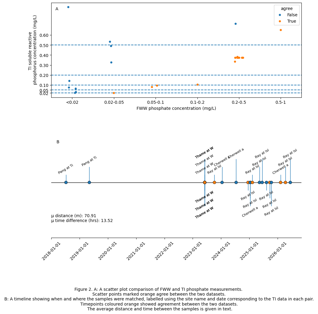
# plot the resultsfig, axes = plt.subplots(nrows=2)# strip plotsns.stripplot(x='fww_value',y='ti_value',data=merged_timeseries_fww_ti_dd, order=["<0.02","0.02-0.05","0.05-0.1","0.1-0.2","0.2-0.5","0.5-1"], hue='agree', ax=axes[0])axes[0].set_xlabel('FWW phosphate concentration (mg/L)')axes[0].set_ylabel('TI soluble reactive \n phosphorus concentration (mg/L)')axes[0].set_yticks([0.02,0.05,0.1,0.2,0.3,0.4,0.5,0.6])axes[0].axhline(y=0.02,ls='--')axes[0].axhline(y=0.05,ls='--')axes[0].axhline(y=0.1,ls='--')axes[0].axhline(y=0.2,ls='--')axes[0].axhline(y=0.5,ls='--')axes[0].text(x=-.4,y=.85,s="A")# timeline# Sort by ti_dtidf = merged_timeseries_fww_ti_dd.sort_values(by='ti_dti')# stagger the stems levels = [1, 2, 3, -1, -2, -3] *len(df)levels = levels[:len(df)]# Draw horizontal lineaxes[1].axhline(0, color='black', linewidth=1)# Draw stems and pointssns.scatterplot(ax=axes[1],x='ti_dti', y=[0]*len(df), hue='agree', s=50, zorder=3,data=df, legend=False, edgecolor='k')ci =0for i in df.index:if pd.notna(df.loc[i,'ti_dti']): axes[1].vlines(df.loc[i,'ti_dti'], 0, levels[ci], linewidth=1) ci +=1# Ensure annotations aren't too longdf['annot'] = df["ti_site"].str.slice(0,10)# Annotate each pointfor d, l, sname, di, hd inzip(df['ti_dti'], levels, df['annot'],df['distance'],df['hours_diff']): di = np.round(di,2) hd = np.round(hd,2) axes[1].text(d, l, f"{sname}", ha='center', va='bottom'if l >0else'top', fontsize=8, rotation=30)# Format x-axisaxes[1].xaxis.set_major_formatter(DateFormatter('%Y-%m-%d'))# Remove y-axis axes[1].get_yaxis().set_visible(False)#remove some spinesaxes[1].spines[["left", "top", "right"]].set_visible(False)axes[1].set_ylim([-7,5])axes[1].set_xticks(ticks=axes[1].get_xticks(),rotation=45,labels=axes[1].get_xticklabels())axes[1].set_xlabel("")axes[1].text(x=axes[1].get_xticks()[0],y=-5,s=f"μ distance (m): { np.round(df['distance'].mean(),2)}\nμ time difference (hrs): { np.round(df['hours_diff'].mean(),2)}")axes[1].text(x=axes[1].get_xticks()[0],y=5,s=f" B")fig.tight_layout()fig.set_size_inches(10,10)fig.text(.5, -.05, "Figure 2. A: A scatter plot comparison of FWW and TI phosphate measurements. \n Scatter points marked orange agree between the two datasets. \n B: A timeline showing when and where the samples were matched, labelled using the site name and date corresponding to the TI data in each pair. \n Timepoints coloured orange showed agreement between the two datasets. \n The average distance and time between the samples is given in text.", ha='center')
Text(0.5, -0.05, 'Figure 2. A: A scatter plot comparison of FWW and TI phosphate measurements. \n Scatter points marked orange agree between the two datasets. \n B: A timeline showing when and where the samples were matched, labelled using the site name and date corresponding to the TI data in each pair. \n Timepoints coloured orange showed agreement between the two datasets. \n The average distance and time between the samples is given in text.')
Code
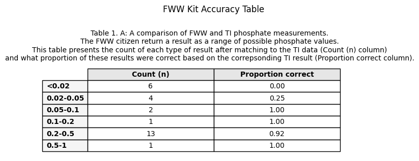
# make a table to show accuracy of different FWW classificationsfig, ax = plt.subplots()# tablesummary = ( merged_timeseries_fww_ti_dd .groupby('fww_value')['agree'] .agg( n='count', proportion_agree='mean' ))order = ["<0.02","0.02-0.05","0.05-0.1","0.1-0.2","0.2-0.5","0.5-1"]summary = summary.reindex(order)table_df = summary.copy()table_df['proportion_agree'] = table_df['proportion_agree'].map('{:.2f}'.format)table_df['n'] = table_df['n'].astype(int)ax.axis('off')ax.set_title("FWW Kit Accuracy Table")tbl = ax.table( cellText=table_df.values, colLabels=['Count (n)', 'Proportion correct'], rowLabels=table_df.index, loc='center', cellLoc='center')# Formattingtbl.auto_set_font_size(False)tbl.set_fontsize(10)tbl.scale(1, 1.4)# Header stylingfor (row, col), cell in tbl.get_celld().items():if row ==0: cell.set_text_props(weight='bold') cell.set_facecolor('#E6E6E6')if col ==-1: # row labels cell.set_text_props(weight='bold') cell.set_facecolor('#F5F5F5')fig.text(.5, .7, "Table 1. A: A comparison of FWW and TI phosphate measurements.\nThe FWW citizen return a result as a range of possible phosphate values.\nThis table presents the count of each type of result after matching to the TI data (Count (n) column)\nand what proportion of these results were correct based on the correpsonding TI result (Proportion correct column).", ha='center')
Text(0.5, 0.7, 'Table 1. A: A comparison of FWW and TI phosphate measurements.\nThe FWW citizen return a result as a range of possible phosphate values.\nThis table presents the count of each type of result after matching to the TI data (Count (n) column)\nand what proportion of these results were correct based on the correpsonding TI result (Proportion correct column).')
Interpretation
We matched 26 samples between FWW and TI datasets, the average spatial distance between the samples was 70 m and average time difference was 13.5 hours. Samples matched from 2018 to 2026, with most samples matching in the period 2023–2026. Samples matched at four sites: Pang at Tidmarsh, Thame at Wheatley, Ray at Islip and Cherwell at Hampton Poyle.
Taking the TI values to be the truth (because they are based on a more accurate lab-based method), when the FWW test kits predict above 0.05 they can generally be trusted with an overally accuracy of 16/17 (94%). However, below 0.05 the prediction accuracy of FWW kits is poor, with an overall accuracy of 1/9 (11%). When compared to the TI dataset, FWW kits have a tendency to underestimate the true phosphate level.
Comparison of EA and FWW Phosphate data
Matching samples
Code
merged_timeseries = pd.DataFrame()for idx in merged_site_wq_fww.index:#download the fww timeseries data response = requests.get(f"https://oxfordrivers.ceh.ac.uk/getTimeseries?siteID={merged_site_wq_fww.loc[idx,'properties.id_right']}&datasetID=freshwater_watch&determinand=chemical_phosphate") fww_timeseries=pd.json_normalize(response.json(), record_path ='data')# format into a dataframeiflen(fww_timeseries) >0: fww_timeseries['dti'] = pd.DatetimeIndex(fww_timeseries['datetime']).tz_convert(None) fww_timeseries['date'] = fww_timeseries['dti'].dt.date fww_timeseries['jul2'] = pd.DatetimeIndex(fww_timeseries['dti']).to_julian_date() fww_timeseries['site'] = merged_site_wq_fww.loc[idx,'properties.id_right'] fww_timeseries['distance'] = merged_site_wq_fww.loc[idx,'distance']# download the ea timeseries data response = requests.get(f"https://oxfordrivers.ceh.ac.uk/getTimeseries?siteID={merged_site_wq_fww.loc[idx,'properties.id_left']}&datasetID=ea_water_quality&determinand=0180") eawq_timeseries=pd.json_normalize(response.json(), record_path ='data')# format into a dataframeiflen(eawq_timeseries)>0: eawq_timeseries['dti'] = pd.DatetimeIndex(eawq_timeseries['datetime']) eawq_timeseries['date'] = eawq_timeseries['dti'].dt.date eawq_timeseries['jul2'] = pd.DatetimeIndex(eawq_timeseries['dti']).to_julian_date() eawq_timeseries['site'] = merged_site_wq_fww.loc[idx,'properties.id_left']#the line below merges the fww and ti data based on time, and ensures dates are no more than one day apart. merged_timeseries = pd.concat([merged_timeseries,pd.merge_asof(fww_timeseries.sort_values('jul2'),eawq_timeseries.sort_values('jul2'), left_on='jul2', right_on='jul2', direction='nearest', tolerance=1)])# calculate the time difference between merged samples merged_timeseries['timedelta'] = merged_timeseries['dti_x'] - merged_timeseries['dti_y']merged_timeseries=merged_timeseries.filter(['value_x','value_y','dti_x','dti_y','site_x','site_y', 'distance', 'timedelta'])merged_timeseries=merged_timeseries.rename(columns={'value_x':'fww_value', 'value_y':'eawq_value','dti_x':'fww_dti','dti_y':'eawq_dti','site_x':'fww_site','site_y':'eawq_site'})merged_timeseries = merged_timeseries[merged_timeseries['eawq_value'].notnull()]merged_timeseries['hours_diff'] =abs(merged_timeseries['timedelta'].dt.total_seconds()/3600)merged_timeseries.reset_index(inplace=True)
Now figure out which FWW measurements match the EA measurements
Code
fwwDictMin = {"<0.02":0,"0.02-0.05": 0.02,"0.05-0.1":0.05,"0.1-0.2":0.1,"0.2-0.5":0.2,"0.5-1":0.5}fwwDictMax = {"<0.02":.02,"0.02-0.05": 0.05,"0.05-0.1":0.1,"0.1-0.2":0.2,"0.2-0.5":0.5,"0.5-1":1}merged_timeseries['agree'] =Falsefor idx in merged_timeseries.index: fwwcat = merged_timeseries.loc[idx,'fww_value']# deal with string ea valuesif merged_timeseries.loc[idx,'eawq_value'] =='<0.01': merged_timeseries.loc[idx,'eawq_value'] =0.01if merged_timeseries.loc[idx,'eawq_value'] >= fwwDictMin[fwwcat] and merged_timeseries.loc[idx,'eawq_value'] <= fwwDictMax[fwwcat]: merged_timeseries.loc[idx,'agree'] =True
Figures and tables
Code
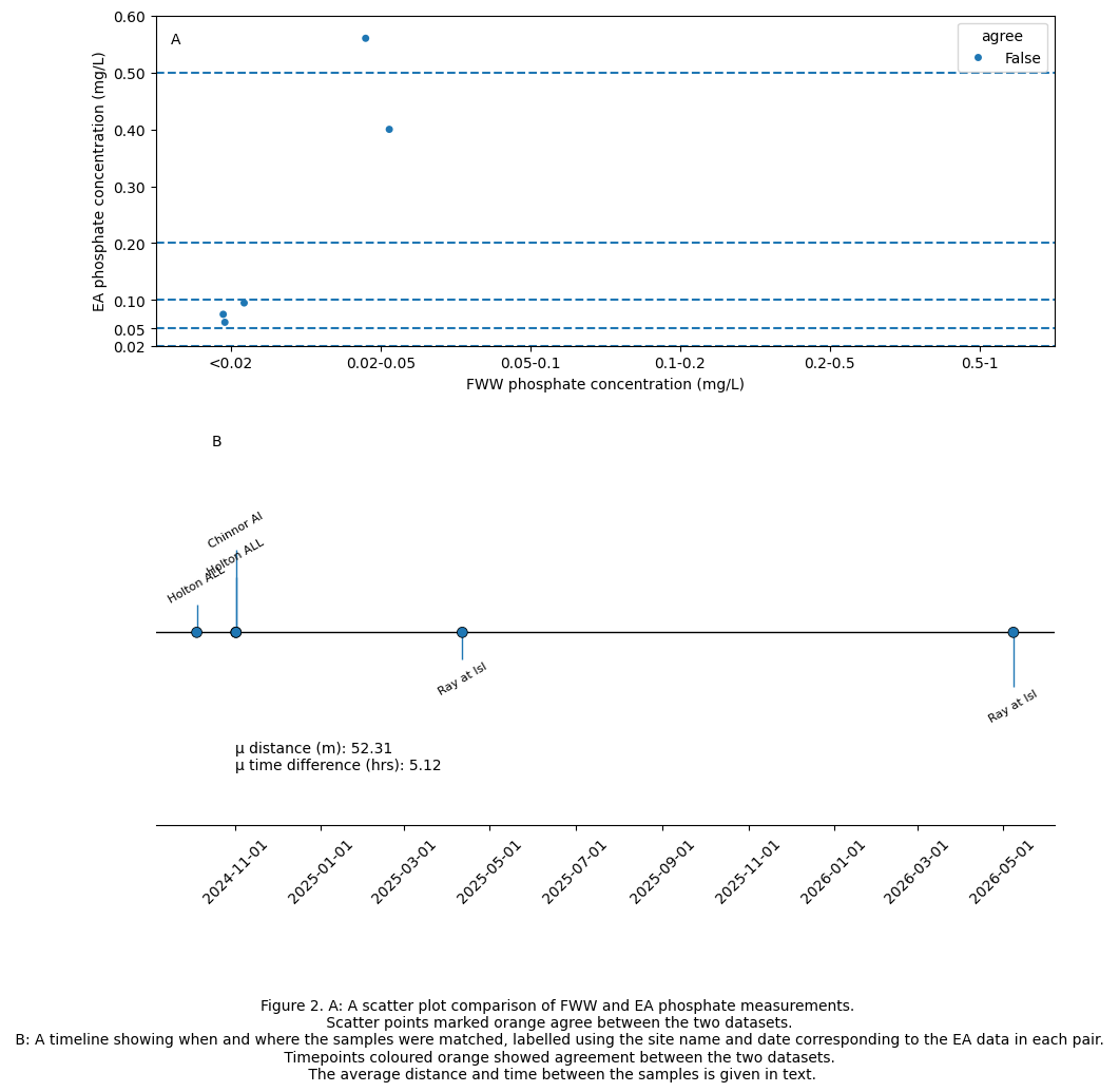
# plot the resultsfig, axes = plt.subplots(nrows=2)# strip plotsns.stripplot(x='fww_value',y='eawq_value',data=merged_timeseries, order=["<0.02","0.02-0.05","0.05-0.1","0.1-0.2","0.2-0.5","0.5-1"], hue='agree', ax=axes[0])axes[0].set_xlabel('FWW phosphate concentration (mg/L)')axes[0].set_ylabel('EA phosphate concentration (mg/L)')axes[0].set_yticks([0.02,0.05,0.1,0.2,0.3,0.4,0.5,0.6])axes[0].axhline(y=0.02,ls='--')axes[0].axhline(y=0.05,ls='--')axes[0].axhline(y=0.1,ls='--')axes[0].axhline(y=0.2,ls='--')axes[0].axhline(y=0.5,ls='--')axes[0].text(x=-.4,y=.55,s="A")# timeline# Sort by ti_dtidf = merged_timeseries.sort_values(by='eawq_dti')# stagger the stems levels = [1, 2, 3, -1, -2, -3] *len(df)levels = levels[:len(df)]# Draw horizontal lineaxes[1].axhline(0, color='black', linewidth=1)# Draw stems and pointssns.scatterplot(ax=axes[1],x='eawq_dti', y=[0]*len(df), hue='agree', s=50, zorder=3,data=df, legend=False, edgecolor='k')ci =0for i in df.index:if pd.notna(df.loc[i,'eawq_dti']): axes[1].vlines(df.loc[i,'eawq_dti'], 0, levels[ci], linewidth=1) ci +=1# Ensure annotations aren't too longdf['annot'] = df["fww_site"].str.slice(0,10)# Annotate each pointfor d, l, sname, di, hd inzip(df['eawq_dti'], levels, df['annot'],df['distance'],df['hours_diff']): di = np.round(di,2) hd = np.round(hd,2) axes[1].text(d, l, f"{sname}", ha='center', va='bottom'if l >0else'top', fontsize=8, rotation=30)# Format x-axisaxes[1].xaxis.set_major_formatter(DateFormatter('%Y-%m-%d'))# Remove y-axis axes[1].get_yaxis().set_visible(False)#remove some spinesaxes[1].spines[["left", "top", "right"]].set_visible(False)axes[1].set_ylim([-7,5])axes[1].set_xticks(ticks=axes[1].get_xticks(),rotation=45,labels=axes[1].get_xticklabels())axes[1].set_xlabel("")axes[1].text(x=axes[1].get_xticks()[0],y=-5,s=f"μ distance (m): { np.round(df['distance'].mean(),2)}\nμ time difference (hrs): { np.round(df['hours_diff'].mean(),2)}")fig.text(x=0.17,y=.55,s="B")fig.tight_layout()fig.set_size_inches(10,10)fig.text(.5, -.05, "Figure 2. A: A scatter plot comparison of FWW and EA phosphate measurements. \n Scatter points marked orange agree between the two datasets. \n B: A timeline showing when and where the samples were matched, labelled using the site name and date corresponding to the EA data in each pair. \n Timepoints coloured orange showed agreement between the two datasets. \n The average distance and time between the samples is given in text.", ha='center')
Text(0.5, -0.05, 'Figure 2. A: A scatter plot comparison of FWW and EA phosphate measurements. \n Scatter points marked orange agree between the two datasets. \n B: A timeline showing when and where the samples were matched, labelled using the site name and date corresponding to the EA data in each pair. \n Timepoints coloured orange showed agreement between the two datasets. \n The average distance and time between the samples is given in text.')
Code
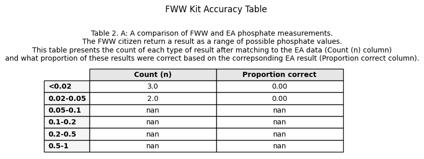
# make a table to show accuracy of different FWW classificationsfig, ax = plt.subplots()# tablesummary = ( merged_timeseries .groupby('fww_value')['agree'] .agg( n='count', proportion_agree='mean' ))order = ["<0.02","0.02-0.05","0.05-0.1","0.1-0.2","0.2-0.5","0.5-1"]summary = summary.reindex(order)table_df = summary.copy()table_df['proportion_agree'] = table_df['proportion_agree'].map('{:.2f}'.format)table_df['n'] = table_df['n'].astype(float)ax.axis('off')ax.set_title("FWW Kit Accuracy Table")tbl = ax.table( cellText=table_df.values, colLabels=['Count (n)', 'Proportion correct'], rowLabels=table_df.index, loc='center', cellLoc='center')# Formattingtbl.auto_set_font_size(False)tbl.set_fontsize(10)tbl.scale(1, 1.4)# Header stylingfor (row, col), cell in tbl.get_celld().items():if row ==0: cell.set_text_props(weight='bold') cell.set_facecolor('#E6E6E6')if col ==-1: # row labels cell.set_text_props(weight='bold') cell.set_facecolor('#F5F5F5')fig.text(.5, .7, "Table 2. A: A comparison of FWW and EA phosphate measurements.\nThe FWW citizen return a result as a range of possible phosphate values.\nThis table presents the count of each type of result after matching to the EA data (Count (n) column)\nand what proportion of these results were correct based on the correpsonding EA result (Proportion correct column).", ha='center')
Text(0.5, 0.7, 'Table 2. A: A comparison of FWW and EA phosphate measurements.\nThe FWW citizen return a result as a range of possible phosphate values.\nThis table presents the count of each type of result after matching to the EA data (Count (n) column)\nand what proportion of these results were correct based on the correpsonding EA result (Proportion correct column).')
Interpretation
We matched 4 samples between FWW and EA datasets, the average spatial distance between the samples was 50 m and average time difference was 2 hours. Samples matched from 2024 to 2025. Samples matched at three sites: Ray at Islip, Holton and Chinnor.
Taking the EA values to be the truth (because they are based on a more accurate lab-based method), the results support our previous finding that below 0.05 the prediction accuracy of FWW kits is poor, with an overall accuracy of 0 out of 4 (0%). Again, when compared to the EA results, we find that the FWW kits have a tendency to underestimate the true phosphate level.
Hypothesis: FWW test kits over report minimal phosphate (< 0.05 mg/L) values because subtle colour changes of test strips are hard to see.
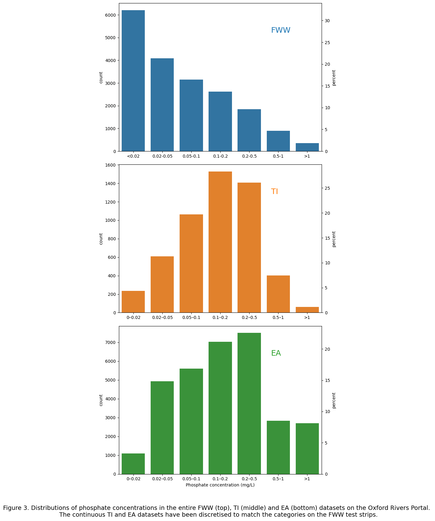
This is supported by the comparisons with regulatory/lab data above, which show the lowest proportion correct when the tests predict < 0.02 mg/L. Let's look at the distributions of phosphate values in the entire datasets that are held for each measuring organisation on the Oxford Rivers Portal to see if the FWW data is more left skewed than the EA and TI data.
Downloading entire datasets
Code
# Download all TI measurementsti_all = []for idx in thamesinit_sites.index:# download the thames initiative time series data for each site response = requests.get(f"https://oxfordrivers.ceh.ac.uk/getTimeseries?siteID={thamesinit_sites.loc[idx,'properties.id']}&datasetID=thames_initiative&determinand=Soluble%20reactive%20phosphorus%20(%CE%BCg/L)") ti_all.append(pd.json_normalize(response.json(), record_path ='data'))# concat it all togetherti_df = pd.concat(ti_all).reset_index()# convert non numerical data to nanti_df['value'] = pd.to_numeric(ti_df['value'], errors='coerce')ti_df['value_mg'] = ti_df['value']/1000# Download all EA measurementsea_all = []for idx in eawq_sites.index:# download the thames initiative time series data for each site response = requests.get(f"https://oxfordrivers.ceh.ac.uk/getTimeseries?siteID={eawq_sites.loc[idx,'properties.id']}&datasetID=ea_water_quality&determinand=0180") ea_all.append(pd.json_normalize(response.json(), record_path ='data'))# concat it all togetherea_df = pd.concat(ea_all).reset_index()# convert non numerical data to nanea_df['value'] = pd.to_numeric(ea_df['value'], errors='coerce')# Download all FWW measurements.fww_all = []for idx in fww_sites.index:# download the thames initiative time series data for each site response = requests.get(f"https://oxfordrivers.ceh.ac.uk/getTimeseries?siteID={fww_sites.loc[idx,'properties.id']}&datasetID=freshwater_watch&determinand=chemical_phosphate") fww_all.append(pd.json_normalize(response.json(), record_path ='data'))# concat it all togetherfww_df = pd.concat(fww_all).reset_index()fww_df['value']=pd.Categorical(fww_df['value'], categories=['<0.02','0.02-0.05','0.05-0.1','0.1-0.2','0.2-0.5','0.5-1','>1','No_water_available',''])fww_df.drop(fww_df[fww_df['value'] =='No_water_available'].index, inplace=True)fww_df.drop(fww_df[fww_df['value'] ==''].index, inplace=True)fww_df['value']=pd.Categorical(fww_df['value'], categories=['<0.02','0.02-0.05','0.05-0.1','0.1-0.2','0.2-0.5','0.5-1','>1'])# Bin EA and TI data so it matches FWWbins = [0, 0.02, 0.05, 0.1, 0.2, 0.5, 1, np.inf]labels = ["0–0.02", "0.02–0.05", "0.05–0.1","0.1–0.2", "0.2–0.5", "0.5–1", ">1"]ea_df["value_bin"] = pd.cut(ea_df["value"], bins=bins, labels=labels)ti_df["value_bin"] = pd.cut(ti_df["value_mg"], bins=bins, labels=labels)
Comparing distributions of entire datasets
Code
# Now make comparing the counts of the relative bins fig, axes = plt.subplots(nrows=3, figsize=(8,16))sns.countplot(data=fww_df,x='value',ax=axes[0])ax02 = axes[0].twinx()sns.countplot(data=fww_df,x='value',ax=ax02, stat='percent')axes[0].set_xlabel("")axes[0].text(s="FWW",x=.75,y=.8,transform=axes[0].transAxes,color='tab:blue', size=18)sns.countplot(data=ti_df,x='value_bin',ax=axes[1],color='tab:orange')ax12 = axes[1].twinx()sns.countplot(data=ti_df,x='value_bin',ax=ax12, stat='percent',color='tab:orange')axes[1].set_xlabel("")axes[1].text(s="TI",x=.75,y=.8,transform=axes[1].transAxes,color='tab:orange', size=18)sns.countplot(data=ea_df,x='value_bin',ax=axes[2],color='tab:green')ax22 = axes[2].twinx()sns.countplot(data=ea_df,x='value_bin',ax=ax22, stat='percent',color='tab:green')axes[2].text(s="EA",x=.75,y=.8,transform=axes[2].transAxes,color='tab:green', size=18)axes[2].set_xlabel("Phosphate concentration (mg/L)")fig.set_tight_layout(tight=True)fig.text(.5, -.05, "Figure 3. Distributions of phosphate concentrations in the entire FWW (top), TI (middle) and EA (bottom) datasets on the Oxford Rivers Portal. \n The continuous TI and EA datasets have been discretised to match the categories on the FWW test strips.", ha='center', size =14)
Text(0.5, -0.05, 'Figure 3. Distributions of phosphate concentrations in the entire FWW (top), TI (middle) and EA (bottom) datasets on the Oxford Rivers Portal. \n The continuous TI and EA datasets have been discretised to match the categories on the FWW test strips.')
Interpretation
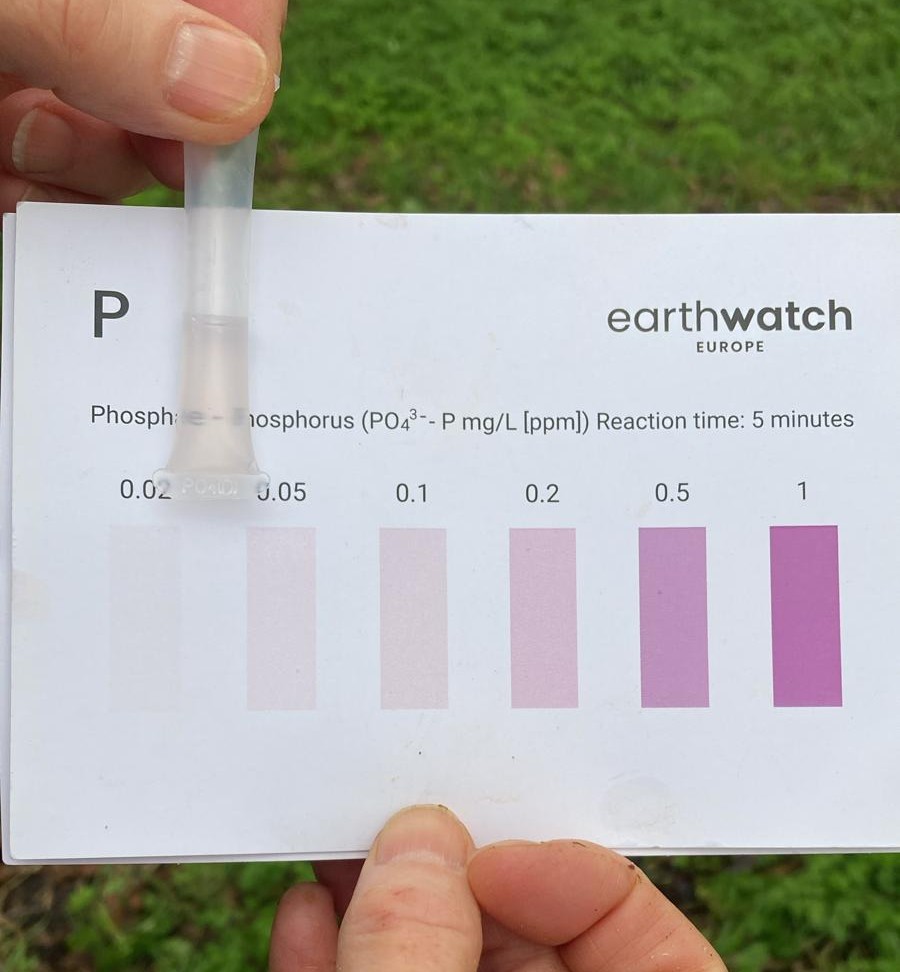
There is an overrepresentation of < 0.02 mg/L measurements in the FWW data compared with the EA and TI. This supports the hypothesis that there is an over representation of 'no colour change' values in the FWW data, because subtle changes in colour denoting concentrations < 0.1 mg/L are hard to see. This explains why there is a large discrepancy between FWW kit measurements and TI/EA measurements when phosphate concentrations are low (e.g. < 0.1 mg/L). An image of FWW testing kit being used in the field a showing a 0.02 - 0.05 mg/L phopshate concentration is shown below. On a cloudy day, or for someone with poorer colour perception than average, this test may be categorised as < 0.02 mg/L.
Conclusion
The TI and EA datasets support each other very well. Overall, the FWW kits seem to be unreliable when they predict low phosphate concentrations ( < 0.05 mg/L) and consistently underestimate the true concentration. However, the FWW kits were found to be more accurate when giving a prediction above 0.05 mg/L. This suggests that if the FWW kits return a high phosphate concentration it is likely to be valid, but if the FWW kits return a low phosphate concentration this cannot necessarily be trusted. One reason for this could be that subtle colour changes in FWW test kits, when concentrations are < 0.05 mg/L, are hard to see, leading to an over representation of the 'no colour change' result. This is supported by highly left skewed distributions of the entire FWW dataset on the Oxford Rivers Portal compared with TI and EA.